In the high-stakes world of optical networking, relying solely on traditional power budget calculations can lead to unforeseen performance bottlenecks. As data centers scale toward 800G and 1.6T, engineers must balance signal integrity with emerging demands for low latency and energy efficiency. This article provides a veteran perspective on how traditional link budgeting compares to modern alternative metrics, helping you optimize for both reliability and cost.
The Fundamentals of Optical Power Budgeting
Defining the Optical Power Budget
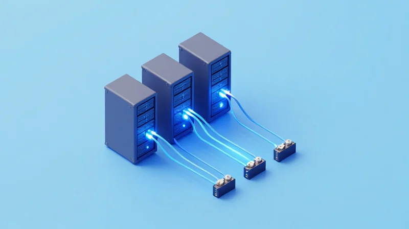
Optical power budgeting is the systematic calculation of the total power loss acceptable within a fiber optic link to guarantee that the signal arriving at the receiver is strong enough to be decoded accurately. It represents the difference between the minimum transmitter output power and the maximum receiver sensitivity, minus various attenuation factors and a dedicated safety margin. Mastering this calculation is the first step in determining whether a proposed network design can physically support the required distance and data rates.
Critical Components of a Link Budget
| Component | Description | Typical Impact |
|---|---|---|
| Transmitter Power (P_tx) | The minimum guaranteed power launched into the fiber. | Starting reference point (dBm). |
| Receiver Sensitivity (P_rx) | The minimum power level required for error-free detection. | Determines the floor (dBm). |
| Fiber Attenuation | Loss per kilometer (varies by wavelength). | Primary distance-based loss. |
| Connector/Splice Loss | Signal drop at physical junctions and patches. | Cumulative discrete losses. |
| System Safety Margin | Buffer for component aging and future repairs. | Standard 3dB to 6dB buffer. |
The Importance of the Safety Margin
A theoretical budget that meets the receiver's threshold exactly is prone to failure in the real world. Engineers apply a safety margin to account for 'unforeseen' variables such as the aging of the laser source, connector contamination over time, and the inevitable addition of splices if a fiber cable is accidentally severed and requires repair. Without this 3dB to 6dB cushion, a link that works perfectly on day one may become unusable within two years.
Manual Calculation vs. Real-time Monitoring Alternatives
| Feature | Traditional Calculation | Real-time Telemetry (Alternative) |
|---|---|---|
| Cost Basis | Fixed Capex (Design phase) | Opex (Ongoing sensor monitoring) |
| Accuracy | Conservative/Theoretical | Actual/Dynamic |
| Risk Management | Reactive (Wait for failure) | Proactive (Detect degradation early) |
| Implementation | Manual planning | Automated software tools |
Frequently Asked Questions
- Why is 1550nm preferred for long-distance budgets?
Wavelengths near 1550nm experience lower attenuation (approx 0.2 dB/km) compared to 1310nm (approx 0.35 dB/km), allowing more power to remain at the end of the link. - Can an optical signal be too strong?
Yes, if the power budget is too 'rich,' it can saturate the receiver (overload), leading to high bit error rates. In these cases, optical attenuators are used to reduce power. - How does connector cleanliness affect the budget?
A single dirty connector can add 1dB or more of loss, potentially consuming the entire safety margin and causing intermittent link drops.
Latency: The Invisible Constraint of Modern Standards

Latency has become the primary constraint in modern optical standards because signal integrity—while necessary—is no longer the sole metric for success in environments where microseconds equate to millions of dollars. Traditional optical power budget calculations focus strictly on ensuring a signal is audible over the noise floor, but they often ignore the processing and propagation delays inherent in complex error-correction schemes and high-density switching fabrics.
The Trade-off: Error Correction vs. Execution Speed
In traditional long-haul or enterprise networking, the priority is maintaining a link margin that can withstand fiber aging and connector degradation. To achieve this at higher speeds like 400G and 800G, standard bodies rely heavily on Forward Error Correction (FEC). While FEC allows for a more relaxed power budget by recovering signals from noisy environments, it introduces a non-negotiable latency penalty. For AI training clusters and High-Frequency Trading (HFT), this 'safe' power budget becomes a performance bottleneck, leading architects to explore alternatives like 'FEC-free' or 'Low-Latency FEC' proprietary links.
| Feature | Power-Centric Design | Latency-Centric Design |
|---|---|---|
| Primary Metric | Decibels (dB / dBm) | Nanoseconds (ns) |
| Signal Recovery | Aggressive FEC (High Latency) | Minimal/No FEC (Direct Drive) |
| Cable Strategy | Standard SMF/MMF Optimization | Shortest Path / Hollow Core Fiber |
| Cost Driver | Optical Amplification/Safety Margin | Specialized Transceivers & ASICs |
Practical Constraints in Modern Architectures
- Does a higher power budget reduce signal delay?
No. While a higher power budget improves the Bit Error Rate (BER), it does not impact the propagation speed of photons or the serialization delay of the hardware. - Why is the traditional safety margin being questioned?
In AI back-end fabrics, engineers often trade the traditional 3dB safety margin for lower-power, simpler modulation schemes that bypass the heavy computational overhead of complex digital signal processing (DSP). - How does fiber length impact the budget vs. latency?
Fiber adds roughly 5ns of latency per meter. While a power budget may support a 10km run, a latency-constrained application might limit that same link to 100 meters to maintain timing sync.
Ultimately, the shift toward latency-aware networking requires a paradigm change. Engineers can no longer simply calculate loss and assume the network is 'fast.' They must now balance the optical power budget against the 'time budget,' ensuring that the methods used to preserve light do not inadvertently destroy the speed of the data it carries.
Power Consumption Analysis: Active vs. Passive Infrastructure
The Energy Trade-off in Optical Network Design
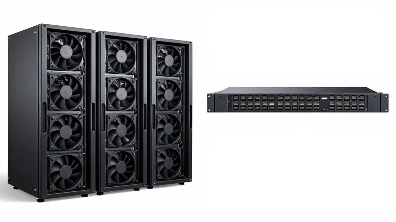
The pursuit of a robust optical power budget often forces a choice between active signal amplification, which requires continuous electrical power and cooling, and passive link optimization, which minimizes power consumption but requires tighter tolerances and superior component quality. While active systems can compensate for significant losses across longer distances, the resulting energy footprint creates a persistent operational expense that passive alternatives can virtually eliminate. In modern data centers, shifting from active regeneration to passive low-loss components is a primary strategy for reducing the Carbon Usage Effectiveness (CUE) of the facility.
Infrastructure Comparison: Power Usage Breakdown
| Infrastructure Type | Key Component | Typical Power Draw | Cooling Requirement |
|---|---|---|---|
| Active | Optical Amplifiers (EDFA) | 15W - 50W per unit | High / Active Fans |
| Active | Transponders/Regenerators | 20W - 100W per card | High / Data Center HVAC |
| Passive | High-Performance Splitters | 0W | None |
| Passive | Low-Loss Connectors | 0W | None |
Operational Impact of Active Signal Regeneration
Active components like Erbium-Doped Fiber Amplifiers (EDFAs) and Optical-Electrical-Optical (OEO) converters are necessary for spanning vast distances, but they introduce a 'power tax.' This tax is not limited to the electricity consumed by the devices themselves; it includes the heat dissipation requirements and the secondary energy used by HVAC systems to maintain optimal operating temperatures. In contrast, passive alternatives focus on reducing the initial insertion loss (IL) of the link through superior materials. By utilizing ultra-low-loss fiber and high-precision connectors, engineers can often achieve the necessary link budget without the need for active, power-hungry equipment, thereby simplifying the thermal management profile of the rack.
Sustainability and Long-Term Scalability
As data centers and AI clusters scale, the cumulative effect of active signal management becomes a bottleneck for sustainability goals. A network relying on passive optimization offers a linear cost model regarding power, whereas active systems introduce exponential complexity as more amplification stages are added to overcome cable degradation or higher port densities. Passive infrastructure also boasts a significantly higher mean time between failures (MTBF), as it lacks the electronic components prone to heat-related degradation. When calculating the Total Cost of Ownership (TCO), the reduction in power consumption often makes passive-first designs the superior choice for high-density environments.
Common Inquiries Regarding Power Efficiency
- Does passive infrastructure always result in lower TCO?
While passive components have zero power draw, the initial capital expenditure for high-quality, ultra-low-loss glass and connectors may be higher. However, the long-term savings in electricity and cooling typically offset these costs within 18 to 36 months of operation. - Can passive alternatives replace amplifiers in long-haul links?
Only to a certain extent. Passive optimization can extend a link's reach by reducing internal loss, but for distances exceeding the physics of the fiber (typically over 80km in standard SMF), active amplification remains a technical necessity. - How does active equipment affect latency compared to passive?
Active equipment often introduces processing or buffering delays, whereas passive components allow for signal transmission at the speed of light within the medium, making passive infrastructure the preferred choice for latency-sensitive applications like HFT.
Signal-to-Noise Ratio (SNR) vs. Power Budgeting

SNR vs. Power Budgeting: The Shift from Quantity to Quality
Traditional power budgeting focuses on ensuring a signal arrives at the receiver with enough decibel (dB) strength to exceed a specific sensitivity threshold. However, in modern 400G and 800G coherent optical systems, raw power is no longer the primary determinant of link success. Instead, Signal-to-Noise Ratio (SNR) and Optical Signal-to-Noise Ratio (OSNR) have become the definitive metrics because they account for the background noise and interference that can corrupt data even if the signal is physically 'loud' enough. While power budgeting measures the volume of the signal, SNR measures its clarity, which is the only way to ensure low Bit Error Rates (BER) in high-density AI and cloud infrastructures.
Key Differences in Performance Management
| Feature | Traditional Power Budgeting | Modern SNR Monitoring |
|---|---|---|
| Primary Metric | Attenuation (dB loss) | Signal Clarity (OSNR/SNR) |
| Main Obstacle | Fiber length and connector loss | Crosstalk, ASE noise, and dispersion |
| Applicability | Legacy 1G to 10G links | High-speed 400G+ coherent links |
| Diagnostic Depth | Basic connectivity (Up/Down) | Predictive reliability and BER trends |
The Noise Floor Problem in High-Speed Links
As data rates increase, the sensitivity of modulation schemes (like 16-QAM or 64-QAM) to noise increases exponentially. In these environments, adding more power to a link can actually be counterproductive. High launch powers can trigger non-linear effects in the fiber, such as Self-Phase Modulation (SPM), which increases the noise floor and effectively lowers the SNR. Effective infrastructure management now requires balancing the power budget to overcome attenuation while simultaneously minimizing noise to maintain the SNR margins required by Forward Error Correction (FEC) algorithms.
Frequently Asked Questions
- Can a link pass a power budget test but still fail to transmit data?
Yes. If the link has high OSNR degradation due to faulty amplifiers or significant crosstalk, the signal may be strong enough for the receiver to detect it, but the noise level will make the data indecipherable. - Why is SNR monitoring considered more cost-effective for large-scale deployments?
SNR monitoring allows for predictive maintenance. By tracking the gradual decline of signal quality against the noise floor, operators can replace components before a total link failure occurs, reducing emergency downtime costs. - Does SNR replace power budgeting entirely?
No; power budgeting is still the foundational step for physical layer design. SNR analysis is an additional, higher-level layer of performance validation required for high-bandwidth standards.
Total Cost of Ownership (TCO) Comparison

Total Cost of Ownership: Rigid Calculation vs. Modern Optimization
Choosing between traditional optical power budget calculations and modern alternatives is fundamentally a decision between paying for 'insurance' in the form of excessive decibel margins or investing in 'intelligence' via real-time monitoring; the former typically results in a 25% to 40% higher TCO due to inflated hardware requirements and energy inefficiencies.
Capital Expenditure (Capex) Drivers
In traditional budgeting models, engineers often select 'worst-case' components to ensure link viability. This leads to the procurement of expensive Extended Reach (ER) or Zephyr Reach (ZR) transceivers even when standard-reach optics, supported by Signal-to-Noise Ratio (SNR) monitoring, would suffice. The cost delta between these transceiver classes can be significant when scaled across a high-density data center or enterprise backbone.
| Cost Factor | Traditional Power Budgeting | Optimized SNR/Alternative Models |
|---|---|---|
| Transceiver Selection | Premium High-Gain (Over-specced) | Standard-Reach (Fit-for-purpose) |
| Infrastructure Complexity | High (Requires more active repeaters) | Low (Focuses on passive link integrity) |
| Deployment Time | Extended (Manual link certification) | Accelerated (Automated validation) |
| Initial Hardware Margin | 5-10 dB (Wasteful buffer) | 2-3 dB (Precision allocation) |
Operational Expenditure (Opex) and Energy Impact
The Opex benefits of alternative strategies are primarily realized through reduced power consumption. Rigid budgets often necessitate active amplification and aggressive cooling for high-power modules. In contrast, optimized architectures prioritize passive components and lower-power transceivers, reducing the carbon footprint and utility costs of the network over a standard 5-to-7-year lifecycle.
- Does reducing the power budget margin increase maintenance costs?
No. By using alternatives like SNR-based monitoring, maintenance becomes predictive rather than reactive, allowing for targeted repairs before a link fails, which reduces emergency truck rolls and downtime costs. - How does hardware longevity factor into TCO?
Traditional budgeting often leads to premature hardware replacement based on conservative age estimates. Alternatives use real-time health data to extend the usable life of optical components, delaying replacement Capex. - What is the impact on energy efficiency?
Optimized alternatives can reduce link-related power draw by 15-20% by eliminating unnecessary active components that were only installed to satisfy a static power budget calculation.
IEEE 802.3 and MSA Standards: A Competitive Landscape
The Interplay of Standards in Optical Power Budgeting
IEEE 802.3 standards act as the regulatory bedrock for optical communications, establishing conservative power budget thresholds to ensure that hardware from disparate vendors remains interoperable under absolute worst-case conditions. While this 'fail-safe' approach guarantees link stability, it often results in over-engineered infrastructure that ignores the efficiencies found in Multi-Source Agreements (MSAs) or proprietary alternative configurations. As data rates climb toward 1.6T, the gap between standard-defined power budgets and real-world performance optimization widens, forcing architects to choose between the safety of strict IEEE compliance and the cost-efficiency of bespoke optical configurations that prioritize Signal-to-Noise Ratio (SNR) over simple decibel loss.
Comparing IEEE 802.3 and MSA Frameworks
| Feature | IEEE 802.3 Standards | MSA (Multi-Source Agreements) |
|---|---|---|
| Primary Goal | Global Interoperability | Rapid Innovation & Cost Reduction |
| Power Budget Margin | High (Conservative) | Optimized (Tight) |
| Technical Focus | Bit Error Rate (BER) & Loss | SNR & Reach Extension |
| Vendor Flexibility | Strictly Regulated | Flexible / Proprietary Extensions |
The Shift Toward SNR-Driven Metrics in Modern Standards
Traditional IEEE power budgeting focuses heavily on decibel loss (dB). However, for 400G and 800G applications, MSAs have pioneered the shift toward using Signal-to-Noise Ratio (SNR) and Transmitter and Dispersion Eye Closure Quaternary (TDECQ) as primary indicators of link health. This alternative landscape allows for longer reaches and thinner power margins by leveraging advanced Forward Error Correction (FEC) and Digital Signal Processing (DSP), effectively bypassing the rigid 'power-in vs. power-out' logic of older standards. By adopting these alternative performance metrics, operators can achieve higher port densities without the thermal and financial penalties of over-provisioning optical power.
Standards and Alternatives FAQ
- Do MSA-compliant transceivers work with IEEE-standard switches?
Yes, most MSAs are built on the foundation of IEEE specifications but refine the optical interface or power consumption targets to meet specific market needs like hyperscale data center density. - Why choose an alternative budget over an IEEE standard?
Alternative budgets are often chosen for large-scale deployments where reducing the power budget margin by even 1dB can lead to significant savings in transceiver costs, cooling, and overall Capex. - Does exceeding IEEE power limits void equipment reliability?
Not necessarily; however, it requires moving from a standard power budget calculation to a comprehensive SNR-based performance analysis to ensure link integrity is maintained via FEC.
Bit Error Rate (BER) and Forward Error Correction (FEC)

The Shift from Decibels to Bit Error Rate (BER)
In legacy optical networking, the primary concern was whether enough photons reached the receiver to distinguish a '1' from a '0'. However, in the era of 400G and 800G coherent optics, signal-to-noise ratio (SNR) and Bit Error Rate (BER) have surpassed simple decibel loss as the primary metrics for link reliability. BER provides a direct measurement of transmission quality, capturing the cumulative impact of attenuation, dispersion, and non-linear effects that a simple power budget calculation often overlooks.
Forward Error Correction (FEC) and Coding Gain
Forward Error Correction (FEC) is the mechanism that allows modern links to operate in high-noise environments. By adding redundant parity bits to the data stream, FEC enables the receiver to correct a specific number of bit errors without requiring retransmission. This creates a 'coding gain'—effectively a virtual expansion of the optical power budget. For instance, an FEC algorithm might allow a link with a poor Pre-FEC BER of 10^-3 to achieve an error-free Post-FEC BER of 10^-15, effectively 'reclaiming' several decibels of margin that would otherwise require expensive optical amplifiers or lower-loss fiber.
| Parameter | No FEC (Legacy) | Hard-Decision FEC | Soft-Decision (SD) FEC |
|---|---|---|---|
| Typical Coding Gain | 0 dB | 6 - 7 dB | 9 - 11+ dB |
| Pre-FEC BER Threshold | 10^-12 | 10^-5 | 10^-2 to 10^-3 |
| Overhead (Redundancy) | 0% | ~7% | 20% - 25% |
| Best Use Case | Short-reach / Low-speed | 10G / 40G Metro | 100G+ Long-Haul |
The Performance vs. Latency Trade-off
While FEC provides a significant performance boost, it is not a 'free' alternative to a robust power budget. The computational overhead of decoding complex SD-FEC algorithms introduces latency, typically in the range of microseconds. In High-Frequency Trading (HFT) or real-time data center interconnects (DCI), engineers may prioritize a tighter physical power budget with 'light' FEC to minimize processing delay, whereas long-haul carriers will always prioritize the maximum coding gain to reduce the number of required regeneration sites.
- Why monitor Pre-FEC BER instead of Post-FEC BER?
Post-FEC BER is often zero until the link is about to fail. Pre-FEC BER acts as an early warning system, showing signal degradation trends before they impact traffic. - How does FEC reduce Total Cost of Ownership (TCO)?
By allowing for higher loss tolerances, FEC reduces the need for mid-span amplification and allows the use of lower-cost optical components, significantly lowering Capex. - Can FEC compensate for a failed power budget?
Only to a point. If the signal falls below the 'FEC limit' or 'cliff,' the error correction fails entirely, resulting in total link loss.
Future-Proofing Your Fiber Strategy
Future-proofing your fiber strategy requires a paradigm shift from simple attenuation-based planning to an integrated performance framework that prioritizes signal quality alongside physical link limits. While optical power budgets remain the foundational baseline for network design, the transition to 400G, 800G, and beyond demands that architects incorporate Bit Error Rate (BER) targets and Forward Error Correction (FEC) gains into the initial design phase. This holistic approach prevents premature infrastructure obsolescence by accounting for the complex trade-offs between optical power, noise, and data throughput in modern coherent systems.
Strategic Integration of Advanced Metrics
As network speeds increase, the reliance on a static link margin becomes a liability. Future-proof strategies utilize a multi-layered verification process. This includes using traditional power budgets to establish physical layer viability, while simultaneously applying OSNR (Optical Signal-to-Noise Ratio) modeling to ensure the link can support the higher baud rates of next-generation transceivers. By shifting focus toward the electrical-to-optical conversion efficiency, operators can extract more value from existing glass before requiring expensive fiber overbuilds.
| Planning Metric | Focus Area | Future-Proofing Benefit |
|---|---|---|
| Optical Power Budget | Physical Loss (dB) | Ensures basic connectivity and link viability. |
| OSNR Analysis | Signal Clarity | Predicts performance for coherent 400G/800G+ links. |
| FEC Margin | Error Correction Capability | Extends reach and lowers Capex on high-end optics. |
| BER Monitoring | Real-time Reliability | Allows for proactive maintenance before link failure. |
Optimizing Capex and Opex through Balanced Design
A future-proof strategy is not necessarily an over-engineered one. Over-provisioning optical power leads to unnecessary Capex through the purchase of high-gain optics and amplification hardware that may never be fully utilized. Instead, leveraging FEC and DSP (Digital Signal Processing) capabilities allows for tighter power budgets, reducing the initial investment. Opex is similarly optimized by using these alternative metrics to create automated monitoring thresholds, reducing the need for manual site visits to troubleshoot signal degradation.
Scalability and Standards Compliance
Adhering to IEEE 802.3 and MSA standards ensures that your performance metrics remain relevant as hardware vendors iterate. A strategy that aligns with these standards while allowing for proprietary FEC enhancements provides the maximum flexibility for future hardware swaps. This approach ensures that as transceivers evolve from 400G-QSFP-DD to 800G and 1.6T formats, the underlying power budget and performance calculations remain a reliable foundation for expansion.
- How does FEC integration change my power budget calculation?
FEC effectively increases the 'allowable' loss by enabling the receiver to correct errors induced by noise, allowing for tighter margins and the use of more cost-effective optics. - When should I transition from power budget-centric to OSNR-centric planning?
This transition is critical when moving to coherent optics and speeds above 100G, where chromatic dispersion and noise become more significant than simple attenuation. - Does future-proofing require higher-grade fiber?
Not necessarily; while low-loss fiber helps, a strategy focused on optimized BER and FEC can often extend the life of existing G.652 fiber plants for much higher speeds.
While the optical power budget remains a cornerstone of fiber design, it is no longer the only metric that matters. By integrating latency, energy efficiency, and SNR into your planning, you can achieve a significantly lower TCO and superior performance. Contact our engineering team today for a comprehensive audit of your optical infrastructure to ensure it meets tomorrow's standards.