In the world of high-speed optical networking, the difference between a high-performing link and a complete system failure lies in the precision of the power budget. As data rates push toward 400G and 800G, understanding the physics of light attenuation and the technical constraints of hardware becomes paramount for network engineers. This guide provides an authoritative deep dive into calculating and managing optical power budgets to ensure seamless connectivity.
Defining the Optical Power Budget
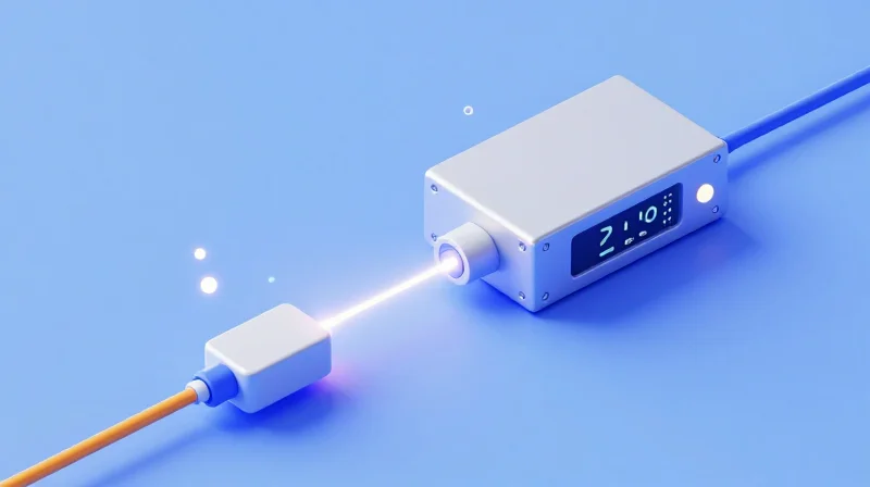
Understanding the Optical Power Budget
An optical power budget represents the total amount of light energy available to a fiber optic system to maintain a functional link between a transmitter and a receiver. It is essentially the strategic allocation of optical power designed to compensate for various attenuation factors and signal degradations—such as fiber attenuation, connector insertions, and splicing losses—while ensuring the signal reaching the photodetector remains within the receiver's operational threshold. Without a properly calculated budget, a network risks intermittent connectivity or total link failure due to signal attenuation or receiver saturation.
The Fundamental Equation
The core of power budgeting lies in a simple subtraction that establishes the total loss permissible across the optical path. By measuring the difference between the source power and the destination's minimum requirements, engineers can define the boundaries of their physical network design.
Power Budget (dB) = Transmitter Output Power (dBm) - Receiver Sensitivity (dBm)Key Components of the Power Budget
| Component | Role in Budgeting | Critical Impact |
|---|---|---|
| Transmitter Power | The starting energy level | Determines the initial 'fuel' available for the link. |
| Receiver Sensitivity | The minimum threshold | Defines the lowest power level for error-free detection. |
| Channel Loss | The sum of all attenuations | The cumulative reduction in signal intensity over distance. |
| Design Margin | The safety buffer | Protects against component aging and future repairs. |
Allocating Power for Signal Integrity
In professional network design, the budget is not just about meeting the minimum sensitivity. It involves a granular breakdown of every potential point of loss. This includes 'link loss,' which covers the fiber medium itself, and 'installation loss,' which accounts for the mechanical aspects of the network. A robust budget also incorporates a safety margin, typically between 3 dB and 6 dB, to account for environmental fluctuations, future splices necessitated by cable breaks, and the natural degradation of laser diodes over time.
Frequently Asked Questions
- What happens if the optical power exceeds the budget?
If the power reaching the receiver is too high, it can saturate the photodetector, leading to high bit-error rates (BER) or physical damage. In such cases, optical attenuators are used to bring the power back into the acceptable range. - How does wavelength affect the power budget?
Different wavelengths experience different attenuation rates. For example, 1310 nm fiber typically has higher loss per kilometer than 1550 nm fiber, meaning the budget must be adjusted based on the specific wavelength used. - Why is a safety margin necessary?
A safety margin ensures that as components age or if the fiber is repaired (adding new splices), the link continues to function without requiring a complete hardware overhaul.
The Core Components of a Power Budget Formula

An optical power budget is fundamentally a mathematical balance sheet that ensures the light signal arriving at the far end of a fiber link remains strong enough for accurate data recovery. By accounting for every decibel of power from launch to reception, engineers can guarantee that the signal-to-noise ratio remains within functional limits, preventing link failures even as components age or environmental conditions fluctuate.
1. Minimum Transmitter Power (PTX_min)
The budget begins at the optical source. The Minimum Transmitter Power represents the lowest guaranteed optical energy an SFP, QSFP, or laser diode launches into the fiber under normal operating conditions. Measured in decibel-milliwatts (dBm), this value is a fixed specification provided by the manufacturer. Professionals must use the minimum rated power rather than the 'typical' or 'average' power to ensure the link calculation accounts for the worst-case hardware performance within manufacturing tolerances.
2. Receiver Sensitivity (PRX_min)
At the opposite end of the link is the receiver sensitivity, which represents the photodetector's detection floor. This is the minimum level of optical power required for the receiver to accurately convert light back into electrical signals while maintaining a specific Bit Error Rate (BER). If the signal arriving at the receiver is weaker than this threshold, the data becomes unreadable. Sensitivity is expressed as a negative dBm value; the more negative the number, the more sensitive (and often more expensive) the receiver.
3. Maximum Allowable Loss (The Power Budget)
The available power budget is the mathematical difference between the transmitter's launch power and the receiver's threshold. This figure represents the total amount of optical attenuation, measured in decibels (dB), that the fiber infrastructure can tolerate. This 'budget' must cover all passive components in the link, including fiber cable distance, connectors, mechanical splices, and fusion splices, while still leaving a safety margin for future repairs or component degradation.
| Variable | Unit | Role in Formula |
|---|---|---|
| Transmitter Power (Min) | dBm | Starting energy level (Source) |
| Receiver Sensitivity | dBm | Minimum required energy (Threshold) |
| Total Power Budget | dB | Total allowable loss (Tx - Rx) |
| Link Loss Margin | dB | Safety buffer for aging and repairs |
Component Selection FAQs
- Why prioritize 'Minimum' Transmitter Power over 'Typical'?
Using minimum values provides a conservative engineering baseline. It ensures that even if you install a transceiver that performed at the bottom of its testing range, the link will not fail. - How does Wavelength impact these components?
While the formula remains the same, the values change. Receivers have different sensitivity levels for 1310nm vs. 1550nm, and fiber attenuation is significantly higher at shorter wavelengths. - What happens if the transmitter is too powerful?
If the received power exceeds the 'Receiver Saturation' point, the detector can be overwhelmed or damaged, requiring the use of an optical attenuator to bring the signal back into a safe range.
Identifying Primary Sources of Signal Attenuation

Identifying the primary sources of signal attenuation is a fundamental requirement for accurate link engineering; it involves isolating the energy loss inherent to the fiber material from the losses introduced by the physical components and environmental stressors within the network path.
Intrinsic Losses: Material and Structural Factors
Intrinsic losses are permanent characteristics of the optical fiber determined during manufacturing. The most prominent factor is Rayleigh scattering, which occurs when light interacts with microscopic density fluctuations in the silica glass, causing the photons to scatter in different directions. Another significant intrinsic factor is absorption, where trace impurities—specifically hydroxyl (OH-) ions—absorb specific wavelengths of light and convert them into heat energy. Because these losses are wavelength-dependent, engineers must use the specific attenuation coefficient (dB/km) relevant to the operating window, typically 1310nm or 1550nm.
Extrinsic Losses: Connectors, Splices, and Bends
Extrinsic losses are introduced by the deployment and termination of the fiber. These are often the most variable elements in a power budget calculation. Insertion loss (IL) at connector interfaces is caused by lateral misalignment, angular tilt, or air gaps between fiber cores. Similarly, splice losses occur at the junctions where two fibers are permanently joined. While fusion splices offer the lowest loss, mechanical splices are more susceptible to refractive index mismatches. Additionally, physical bending—categorized as macro-bending (visible loops) and micro-bending (microscopic imperfections in the cladding)—can cause light to leak out of the core, drastically increasing attenuation.
| Loss Component | Typical Loss Range (dB) | Primary Contribution Factor |
|---|---|---|
| Connector Pair | 0.20 to 0.75 dB | Surface contamination or physical misalignment |
| Fusion Splice | 0.01 to 0.10 dB | Core eccentricity or improper arc power |
| Mechanical Splice | 0.20 to 0.50 dB | Index-matching gel degradation |
| Fiber Span (SMF) | 0.20 to 0.35 dB/km | Rayleigh scattering and material absorption |
Common Questions on Signal Attenuation
- How does dust affect the power budget?
Dust particles on a connector end-face can scatter or absorb light, potentially adding several decibels of loss or even damaging the fiber surface through high-power 'pitting'. - Why is 1550nm loss lower than 1310nm loss?
1550nm sits in the 'third window' of optical transmission where Rayleigh scattering is significantly lower than at shorter wavelengths, allowing for longer transmission distances. - What is the impact of fiber aging?
Over time, environmental factors like hydrogen ingress or moisture can cause 'water peaks' in the attenuation spectrum, increasing the overall loss coefficient of the glass.
The Mathematical Framework for Link Loss Budgeting
The Mathematical Equation for Total Link Loss
The core of optical power budget calculation is a deterministic mathematical framework that sums every discrete source of signal reduction across the physical layer. This calculation determines the Total Link Loss (LL), which must be lower than the available power budget to ensure the receiver can decode the signal without errors. The standard formula is expressed as: Total Loss (dB) = (Fiber Length × Attenuation Coefficient) + (Number of Connectors × Connector Loss) + (Number of Splices × Splice Loss) + Design/Repair Margin.
Variable Definitions and Standard Values
| Component | Variable Symbol | Industry Standard Value (SMF) |
|---|---|---|
| Fiber Attenuation | α (dB/km) | 0.35 dB @ 1310nm / 0.22 dB @ 1550nm |
| Connector Loss | Lc (dB) | 0.50 dB to 0.75 dB per pair |
| Splice Loss | Ls (dB) | 0.05 dB to 0.10 dB per splice |
| Repair Margin | M (dB) | 2.0 dB to 5.0 dB (Safety Buffer) |
Step-by-Step Calculation Breakdown
To perform a precise calculation, engineers must account for four distinct segments of the optical path. First, multiply the physical length of the fiber cable in kilometers by the attenuation coefficient specific to the wavelength being used. Second, identify every connector pair (typically at the patch panels) and assign a loss value based on the connector type (e.g., LC/UPC). Third, calculate loss from fusion splices, which occur at cable junctions or repair points. Finally, add a repair margin to account for future cable cuts, component aging, and environmental degradation.
Total_Loss = (L * α) + (N_c * L_c) + (N_s * L_s) + MPractical Loss Budgeting FAQ
- Why is wavelength critical in the math?
The attenuation coefficient (α) changes based on the wavelength of light. For instance, 1310nm light experiences higher glass absorption (approx 0.35 dB/km) than 1550nm light (approx 0.22 dB/km). - What constitutes a 'Connector Pair'?
A connector pair refers to the junction where two connectors meet via an adapter, such as a patch cord plugging into a bulkhead. Each pair typically adds 0.5 dB to 0.75 dB to the budget. - How much margin should be included?
Most network architects include a 2 dB to 3 dB margin for standard enterprise links. For long-haul outdoor fiber, a 5 dB margin is safer to account for multiple future fusion splices resulting from accidental cable cuts.
By applying this framework, operators can establish a 'Maximum Allowable Loss.' If the calculated total loss exceeds the difference between the transmitter's minimum output and the receiver's minimum sensitivity, the network will require higher-power optics or mid-span amplification.
The Role of the System Operating Margin

The Role of the System Operating Margin
The system operating margin (SOM), also known as the safety margin or design buffer, is the dedicated 'extra' power built into an optical link calculation to ensure the network remains operational under sub-optimal conditions. In optical engineering, calculating a link that barely meets the receiver sensitivity threshold is considered a failure in design. Instead, a robust margin—typically between 2 dB and 4 dB—is applied to ensure that the bit error rate (BER) remains within acceptable limits even as the physical plant and active hardware components degrade over their multi-year service life.
Mitigating Hardware Aging and Environmental Factors
Optical performance is not static; it is subject to the predictable decline of semiconductor materials and the unpredictable nature of the environment. Over time, the laser diodes within transmitters lose efficiency, resulting in a lower output power. Similarly, photodetectors in receivers may experience a drift in sensitivity. Beyond hardware aging, environmental shifts such as extreme temperature cycles can cause micro-bends in the fiber or mechanical stress on connectors. The operating margin absorbs these variations, preventing transient outages during peak summer heat or the inevitable end-of-life decline of the transceiver modules.
| Network Scenario | Typical Margin (dB) | Key Considerations |
|---|---|---|
| Short-Range (Intra-DC) | 1.0 - 2.0 dB | Controlled environment, low probability of fiber damage. |
| Enterprise / Campus | 2.0 - 3.0 dB | Variable temperatures, moderate maintenance access. |
| Long-Haul / Outside Plant | 3.0 - 5.0 dB | High risk of fiber cuts, aging, and extreme weather. |
Accounting for Future Maintenance and Repairs
One of the most practical reasons for maintaining a healthy operating margin is to accommodate future physical repairs. If a fiber cable is accidentally severed, the resulting repair will require at least two additional splices or a new patch segment. Each mechanical or fusion splice introduces a specific amount of insertion loss (typically 0.1 to 0.3 dB). If a design has zero margin, the very first repair would exceed the power budget and break the link. By allocating a 3 dB margin, the network designer essentially 'pre-approves' the loss from approximately 10 to 15 future splices, ensuring the infrastructure remains resilient over decades.
- Is a 3 dB margin always required?
While 3 dB is the industry standard 'rule of thumb,' the specific margin should be based on the risk profile of the link and the expected lifespan of the hardware. - What happens if the margin is too high?
Excessive margins can lead to receiver saturation if the signal is too strong, potentially requiring the installation of optical attenuators to protect the photodetector. - Does the margin cover fiber cleaning issues?
Partiality. While a margin helps, it is not a substitute for proper fiber hygiene; dirty connectors can easily exceed a 3 dB loss, bypassing even the best safety buffers.
Impact of Fiber Type and Wavelength on Budgeting
The fundamental variables in any power budget are the fiber type and the wavelength of light being transmitted, as these factors determine the baseline attenuation rate and the maximum achievable link distance. While Singlemode fiber (OS2) is designed for long-reach applications with extremely low loss at 1310nm and 1550nm, Multimode fiber (OM3/OM4/OM5) is optimized for short-reach, high-bandwidth applications where attenuation is significantly higher at the 850nm window.
Wavelength-Dependent Attenuation Profiles
Attenuation in optical fiber is not constant; it fluctuates based on the wavelength of the light source. This phenomenon is primarily due to Rayleigh scattering and absorption. Shorter wavelengths (850nm) encounter more scattering, leading to higher decibel loss per kilometer, whereas longer wavelengths (1550nm) reside in the 'lowest loss' window of silica glass.
| Fiber Category | Wavelength (nm) | Max Attenuation (dB/km) | Primary Use Case |
|---|---|---|---|
| Multimode (OM3/OM4) | 850 nm | 3.0 - 3.5 | Data Centers / Short Reach |
| Multimode (OM3/OM4) | 1300 nm | 1.0 - 1.5 | Legacy LAN Backbones |
| Singlemode (OS2) | 1310 nm | 0.35 - 0.4 | Campus / MAN / Long-haul |
| Singlemode (OS2) | 1550 nm | 0.22 - 0.25 | Ultra Long-haul / DWDM |
Singlemode vs. Multimode: Budgeting Priorities
When budgeting for Multimode systems, engineers must account for modal dispersion, which limits bandwidth over distance. In contrast, Singlemode power budgets are almost exclusively concerned with attenuation and chromatic dispersion. Because Singlemode transceivers use more precise lasers (DFB or VCSEL), they can drive signals much further, but they require a more stringent budget for connector cleanliness due to the smaller core size (9 microns vs 50 microns).
The OM5 Factor and Wideband Budgeting
OM5 fiber, or Wideband Multimode Fiber (WBMMF), introduces a new budgeting dynamic. It is designed to support Shortwave Wavelength Division Multiplexing (SWDM), which uses four wavelengths across the 850nm to 950nm range. When calculating a budget for OM5, the engineer must ensure the power margin is sufficient for the 'worst-case' wavelength in that range, typically at the 950nm end where attenuation differs slightly from the standard 850nm specification.
Frequently Asked Questions
- Why is 1550nm preferred for the longest distances?
1550nm experiences the lowest attenuation in silica glass (approx. 0.22 dB/km), allowing signals to travel the furthest before requiring amplification compared to 1310nm or 850nm. - Does the fiber type change the connector loss allowance?
Technically, TIA/EIA standards allow 0.75 dB per connector for both, but Singlemode budgets often assume a tighter 0.2 dB to 0.5 dB loss to maximize the link distance. - How does wavelength impact the link margin?
Lower wavelengths (850nm) consume the power budget faster. A 500-meter run at 850nm might lose 1.75 dB just in fiber attenuation, while the same run at 1550nm would lose only 0.11 dB.
High-Speed Networking Constraints: Dispersion vs. Power
High-Speed Networking Constraints: Dispersion vs. Power
In high-speed networking environments—specifically 100G, 400G, and 800G—the optical power budget is no longer the sole arbiter of link success. While a power budget calculation might show a positive margin, signal distortion caused by dispersion can render the data unreadable by the receiver. This occurs because higher bit rates utilize shorter pulse durations, making the signal significantly more sensitive to temporal spreading, where bits begin to overlap and create errors before the light ever becomes too dim to detect.
The Dispersion Penalty in Single-Mode Fiber
In Single-mode (OS2) fibers, Chromatic Dispersion (CD) is the primary non-power constraint. CD occurs because different wavelengths of light travel at slightly different speeds through the glass. In 100G+ systems using PAM4 modulation, the pulse intervals are extremely tight. Even minor spreading causes Inter-Symbol Interference (ISI), where the 'tail' of one pulse bleeds into the next. This creates a 'dispersion penalty,' effectively reducing the usable power budget because the receiver requires a higher Signal-to-Noise Ratio (SNR) to distinguish between these distorted pulses.
| Constraint Type | Primary Cause | Impact on 100G+ Links | Mitigation Strategy |
|---|---|---|---|
| Attenuation (Power) | Fiber length, connectors, splices | Signal becomes too faint to detect | Optical amplifiers, high-gain optics |
| Chromatic Dispersion | Wavelength-dependent speeds | Pulse spreading and ISI | DSP, Coherent optics, specialized fiber |
| Modal Dispersion | Multiple light paths in MMF | Severe bandwidth-distance limits | OM5 fiber, VCSEL optimization |
Beyond Power: The Shift to Coherent Detection
To combat dispersion without being limited by the raw power budget, modern long-reach 100G/400G systems have moved from 'Direct Detect' to Coherent Detection. Coherent optics utilize Digital Signal Processing (DSP) to mathematically reconstruct the signal and compensate for chromatic and polarization mode dispersion (PMD) in real-time. This shift means that for many high-speed long-haul applications, engineers prioritize the Optical Signal-to-Noise Ratio (OSNR) over the traditional power loss calculation, as the DSP can 'clean up' a signal that would otherwise be lost to dispersion.
Dispersion vs. Power FAQ
- Can a link fail if the power budget is within limits?
Yes. If the dispersion exceeds the receiver's tolerance (measured in ps/nm), the bit error rate (BER) will rise until the link drops, even if the received power level is high. - Why is dispersion more critical at 100G than 10G?
At 100G, pulses are sent much faster and are narrower. At these speeds, even a tiny amount of temporal spreading causes pulses to overlap, which is less of an issue at slower 10G speeds. - Does Forward Error Correction (FEC) help with dispersion?
Yes, FEC improves the coding gain, allowing the system to recover data from a signal degraded by both power loss and dispersion-induced noise.
Practical Testing and Verification Tools
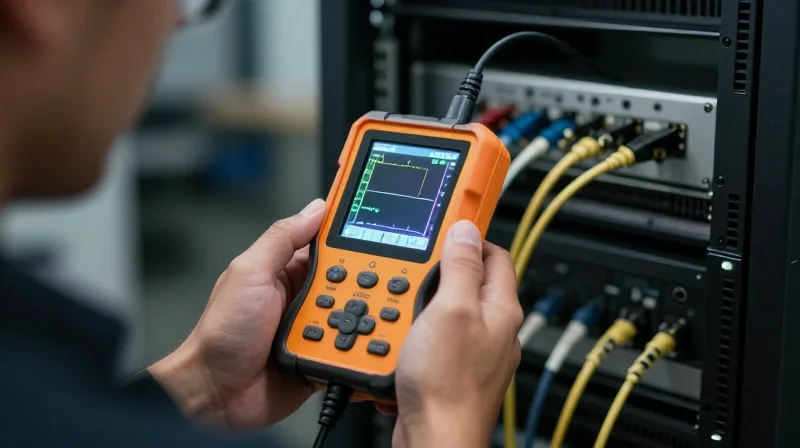
Bridging the Gap Between Theory and Reality
Calculating an optical power budget is a predictive exercise; however, the actual performance of a fiber link can only be validated through standardized field testing. Environmental factors, installation quality, and micro-variations in component manufacturing often lead to discrepancies between paper models and real-world attenuation. Verification tools ensure that the link remains within its operational window, preventing premature hardware failure and ensuring that the safety margin (buffer) remains intact over the link's lifecycle.
The Optical Loss Test Set (OLTS): Tier 1 Certification
The OLTS is the most accurate tool for measuring total end-to-end insertion loss. It utilizes a stabilized light source on one end and a calibrated power meter on the other. This process, often referred to as Tier 1 testing, provides a definitive 'pass/fail' result based on the pre-calculated budget. Because it measures total loss directly, it is the industry standard for certifying that a new installation meets its design specifications.
The Optical Time Domain Reflectometer (OTDR): Tier 2 Troubleshooting
While an OLTS provides a single loss value, an OTDR provides a visual 'trace' of the entire fiber run. By sending high-power pulses and measuring the backscattered light, it identifies the exact location and loss of every splice, connector, and bend. This is classified as Tier 2 testing and is critical for identifying specific points of failure that cause a link to exceed its power budget, such as a contaminated connector or a sharp macro-bend in a patch panel.
| Feature | OLTS (Tier 1) | OTDR (Tier 2) |
|---|---|---|
| Primary Purpose | Measure total insertion loss | Identify event locations and loss values |
| Accuracy | Highest accuracy for total loss | Lower accuracy for total loss due to backscatter estimation |
| Ease of Use | Simple, automated operation | Requires expert interpretation of traces |
| Visual Output | Numeric value (dB) | Graphical trace (distance vs. power) |
| Best For | Standard certification | Troubleshooting and mid-span analysis |
Common Verification Challenges
- Is an OTDR enough for certification?
No. While an OTDR is excellent for characterization, most standards (like TIA-568) require an OLTS for primary certification because the OTDR uses a mathematical approximation of loss rather than a direct power measurement. - What is 'Reference Method' testing?
This involves 'zeroing out' the test leads before measurement. Using the 1-jumper reference method is preferred as it includes the loss of the connections at both ends of the link in the final measurement. - Why does my test show higher loss than my calculation?
Common culprits include dirty connector end-faces, mismatched fiber types (e.g., mixing OM3 and OM4), or exceeding the minimum bend radius during installation, all of which introduce 'hidden' attenuation.
By combining the precision of an OLTS with the diagnostic depth of an OTDR, network engineers can guarantee that their power budget calculations are not just theoretical goals, but operational realities that support reliable high-speed data transmission.
Troubleshooting Common Power Budget Failures
Troubleshooting Common Power Budget Failures
Troubleshooting optical power budget failures requires a systematic approach to isolate whether a 'Link Down' status stems from excessive attenuation, transceiver mismatch, or physical layer degradation. When the measured path loss exceeds the calculated link budget, engineers must look beyond total loss and analyze specific events along the fiber span to identify points of failure that deviate from initial design specifications. Effectively diagnosing these issues ensures that high-speed networks maintain the required Bit Error Rate (BER) performance.
Identifying Root Causes of Excess Attenuation
| Failure Type | Common Symptom | Diagnostic Indicator |
|---|---|---|
| Dirty Connectors | High localized loss & high back-reflection | Visual artifacts on a 400x fiber inspection scope |
| Micro-bends | Wavelength-dependent loss spikes | Significantly higher loss at 1550nm vs 1310nm |
| Transceiver Aging | Low Launch Power (Tx) | DOM/DDM readings below manufacturer specs |
| Core Mismatch | High coupling loss at connections | One-way 'gain' or excessive loss on OTDR trace |
The Impact of Micro-bends and Macro-bends
Physical stress on the fiber, often caused by over-tightened cable ties or improper bend radii in patch panels, induces micro-bends and macro-bends. These stressors allow light to escape the core into the cladding, rapidly depleting the power budget. A professional diagnostic tip is the 'dual-wavelength test': because longer wavelengths are more sensitive to bending loss, a link that passes at 1310nm but fails at 1550nm is a definitive indicator of a physical bend issue rather than contamination.
Practical Diagnostic Steps
- Inspect and Clean
Utilize a fiber inspection probe to verify that all end-faces meet IEC 61300-3-35 standards. Dust is the leading cause of power budget failure. - Verify Transceiver Metrics
Access the Digital Optical Monitoring (DOM) data via the switch CLI to compare real-time Tx/Rx power levels against the calculated threshold. - Perform Tier 1 Testing
Use an Optical Loss Test Set (OLTS) to measure the total end-to-end loss and compare it against the theoretical budget. - Pinpoint with OTDR
If loss is excessive, use an Optical Time Domain Reflectometer (OTDR) to locate the exact meter-mark of high-loss events or reflective splices.
Troubleshooting FAQ
- What if the power is within range but the link still fails?
This often indicates high back-reflection (Return Loss) or dispersion issues. Check for non-angled connectors (UPC) where APC is required, or verify if the fiber length exceeds dispersion limits. - Why does my link work intermittently?
Intermittent failures are typically caused by marginal power budgets where small temperature fluctuations or mechanical vibrations push the Rx power below the sensitivity threshold.
Calculating an accurate optical power budget is not just a best practice—it is a technical necessity for modern enterprise and data center networks. By meticulously accounting for every decibel of loss and maintaining a healthy operating margin, you ensure a robust infrastructure capable of supporting tomorrow's bandwidth demands. Ready to optimize your fiber plant? Contact our engineering team today for a comprehensive network audit and high-performance optical solutions.